

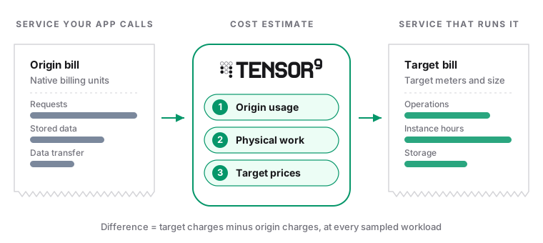
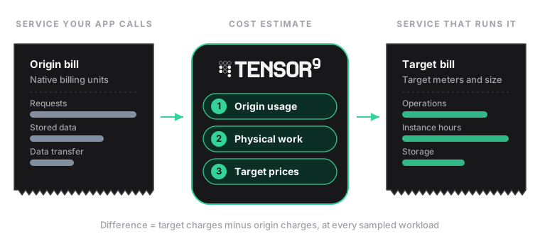
How Tensor9 estimates adapted-service costs
1
Origin usage
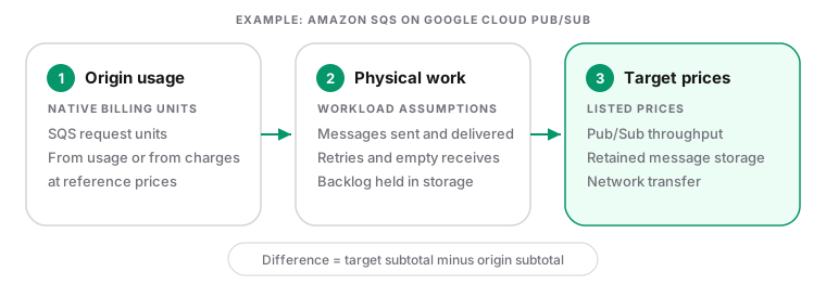
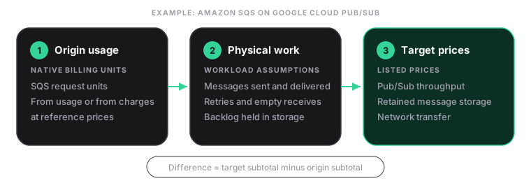
The estimate starts from the origin service’s native billing quantities: SQS 64-KiB request units, DynamoDB read and write request units, S3 GB-months and request counts. State usage directly, or state monthly charges at the model’s reference rates and let the model divide each charge by its rate.
2
Physical work
Workload assumptions translate billing units into the operations, bytes and retained data the target service meters. Message size and batch fill set how many messages a number of SQS request units represents; item size and read consistency set how many point reads a number of DynamoDB read units represents. Every assumption is listed beside the result and can be changed.
3
Target prices
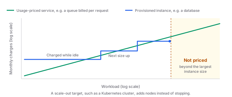
Each target meter is priced at the model’s rates. A provisioned target, such as a database instance, is priced for its selected size for 730 hours per month, whatever the traffic.
Reference rates and planning estimates
Each model states which kind of estimate it is.
Neither kind predicts your invoice.
What the estimates include
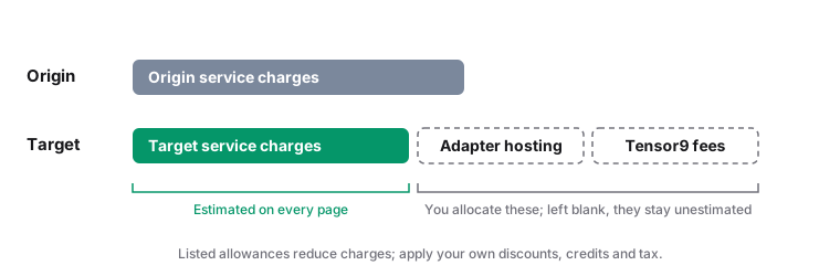
Because the estimates leave out Tensor9 fees and adapter hosting, a lower target subtotal is not a savings figure. A modeled adapted total exists only after both allocations are supplied.
Usage charges and provisioned capacity
Read the cost curves
Each service page and cost guide shows curves without entering usage or uploading a report. A curve varies one named workload dimension, such as message rate or stored data, and keeps the other assumptions fixed in its assumption table.- Axes. Workload and cost axes are logarithmic so several orders of magnitude stay readable. Equal distance means proportional growth; zero has a separate endpoint when present.
- Lines. The dashed line is the origin service. Each colored line is a target configuration. Lines connect evaluated samples; intermediate points, break-even behavior and capacity are not inferred.
- Rows beside the chart. One row per service gives its monthly charge and the difference at the named workload.
- Comparison label. Costs More and Costs Less hold at every sampled point. Costs The Same means within the stated tolerance at every point. Costs Depend covers mixed results and unpriced samples.
- Tables. The table under each curve lists the exact sampled charges and the target-minus-origin difference. Use it rather than the chart for comparisons.
Estimate your own workload
The curves and examples use reference workloads. The monthly cost calculator evaluates the same models with your inputs and returns the same line items, subtotals, qualifications and exclusions. Ask your Tensor9 contact or [email protected] for calculator access or for an estimate of your workload. The calculator accepts three kinds of input:- Usage report. For models that support it, upload an AWS Cost and Usage Report (CUR or CUR 2.0) as an uncompressed CSV file of at most 4 MiB. Tensor9 processes the report in memory and does not save it. Review the recognized meters, period, region and excluded rows, supply any missing meters, and confirm that the report covers a complete month for the selected service before applying it.
- Usage entered by hand. Enter native monthly quantities, such as SQS request units or DynamoDB read and write request units.
- Charges entered by hand. Enter monthly origin charges at list price. The model divides each charge by its reference rate to recover usage, so a discounted or credited total understates the workload.
Review assumptions with a support agent
Ask the agent to separate measured inputs from assumptions and show which changes affect the estimate most. For SQS, for example, message size, batch fill, empty receives and redelivery can change the relationship between application traffic and billed units. A lower modeled subtotal is a hypothesis to test against that workload. Provide a reviewed selection of usage and configuration evidence. A billing report can reveal account identifiers, resource names and business activity. Approval to use the calculator does not authorize sending its report to a model or sharing it with another participant. Use the input and processing controls in Agents and Permissions.Validate the estimate against observed work
Use Tuning with Agents to define a bounded comparison before changing capacity or moving traffic. Record the model inputs and expected cost drivers, then measure completed work, correctness, retries, latency and native usage for the same workload. Compare the matching billing period and resource scope, and account for hosting, Tensor9 fees and other excluded costs separately. Keep estimate and observation labeled separately. A modeled instance size is not proof of achieved capacity, and a successful test is not a complete monthly invoice. If the result differs, investigate the assumptions and metered operations with the support agent before claiming savings. Use Operations with Agents for any resulting resource change, including its owner, spending approval, verification and recovery procedure.Read the qualifications
Every result lists the statements that limit it. Read them before comparing totals.- Rate snapshot, List prices read or Planning assumptions authored gives the date of the rates: a provider rate snapshot, the date cited list prices were read, or the date authored estimates were written. Do not apply them to another region or service tier.
- Designed mapping means the cost model describes an intended adapter. A price does not make that backend available.
- Native or deployment mapping means the cost covers the selected service resources, not request-level operation coverage.
- Estimated allocation from planning assumptions; not benchmark calibrated marks instance sizes chosen by a planning policy rather than measured capacity.
- Unpriced means the workload exceeds a documented limit of the target, named in the result; the difference is then Unavailable.
- Unestimated components lists allocations, such as adapter hosting and Tensor9 fees, that the total does not include.
- Cost scope and Excluded costs and workload features state exactly which charges the subtotals cover.
- A benchmark plan lists planned measurement cases. Planned cases are not completed measurements and do not qualify capacity.
Worked examples
Each example evaluates a published model’s reference workload when this page is generated, so its figures change when the models or their rates change.DynamoDB on Firestore
A DynamoDB Standard on-demand table serving point reads and plain item writes, with retained table data. Monthly AWS usage charges at the 2026-10-18 reference list rates in us-east-1, before free allowances, discounts, credits and tax. For this reference workload, DynamoDB service charges are USD 43.75 per month and Firestore service charges are USD 54.00 per month. Firestore costs USD 10.25 more per month. Step 1: origin usage. The example enters monthly origin charges at list price, and the model divides each charge by its reference rate to recover native usage:- DynamoDB on-demand reads: 12.5 USD/month
- DynamoDB on-demand writes: 6.25 USD/month
- DynamoDB Standard storage: 25 USD/month
Step 2: physical work. These workload assumptions translate the billing units into the work the target service meters:
Implied usage:
- Inferred point reads: 100,000,000 calls/month
- Inferred base item writes: 10,000,000 calls/month
- Origin billed storage: 100 GiB-month
Step 4: comparison.
Across the Monthly cost by DynamoDB point-read rate curve, the difference for the target scenario (Firestore: point reads and blind writes) moves from USD -9.47 per month at 1 reads/s to USD +5311.70 per month at 10,000 reads/s. The Amazon DynamoDB cost guide plots every backend across that range.
Every published backend for DynamoDB, each at one sampled workload from its own cost curve:
Qualifications for this example:
- Firestore Standard edition, regional us-central1. One document read per origin point read; explicit reads/writes per write.
- Plain unconditioned PutItem can use the blind write path; read-modify-write, conditions and retries increase document reads.
- Equal physical storage is an illustrative assumption; tagged item envelopes, metadata and indexes can change billed bytes.
dynamodb-firestore version 2026-10-18.4, scenario dynamodb-firestore-reference.
SQS (Simple Queue Service, Classic) on Pub/Sub
A Standard SQS queue whose messages are sent, received and deleted with the batch fills listed below. Monthly AWS usage charges at the 2026-10-18 reference list rates in us-east-1, before free allowances, discounts, credits and tax. For this reference workload, SQS (Simple Queue Service, Classic) service charges are USD 120.00 per month and Pub/Sub service charges are USD 7.92 per month. Pub/Sub costs USD 112.08 less per month. Step 1: origin usage. The example enters monthly origin charges at list price, and the model divides each charge by its reference rate to recover native usage:- Standard SQS requests: 120 USD/month
Step 2: physical work. These workload assumptions translate the billing units into the work the target service meters:
Implied usage:
- Inferred original messages: 100,000,000 messages/month
Step 4: comparison.
Across the Monthly cost by SQS request rate curve, the difference for the target scenario (one subscription) moves from USD -0.98 per month at 1 requests/s to USD -29455.61 per month at 30,000 requests/s. The Amazon SQS cost guide plots every backend across that range.
Every published backend for SQS (Simple Queue Service, Classic), each at one sampled workload from its own cost curve:
Qualifications for this example:
- One pull subscription, Standard SQS semantics compatible with this mapping, representative message size and batching.
- Pub/Sub publish and delivery each cost USD 40/TiB, with a 1,000-byte minimum per request. Metadata overhead is an explicit assumption.
sqs-pubsub version 2026-10-18.4, scenario sqs-pubsub-reference.
S3 on Cloud Storage
An S3 Standard bucket with retained objects, ordinary PUT requests and ordinary GET requests. Monthly AWS usage charges at the 2026-10-18 reference list rates in us-east-1, before free allowances, discounts, credits and tax. For this reference workload, S3 service charges are USD 244.52 per month and Cloud Storage service charges are USD 213.80 per month. Cloud Storage costs USD 30.72 less per month. Step 1: origin usage. The example enters monthly origin charges at list price, and the model divides each charge by its reference rate to recover native usage:- S3 Standard storage: 235.52 USD/month
- S3 PUT requests: 5 USD/month
- S3 GET requests: 4 USD/month
Step 2: physical work. These workload assumptions translate the billing units into the work the target service meters:
Implied usage:
- Origin retained data: 10,240 GiB-month
- Inferred ordinary PUTs: 1,000,000 requests/month
- Inferred ordinary GETs: 10,000,000 requests/month
Step 4: comparison.
Across the Monthly cost by retained S3 Standard data curve, the difference for the target scenario (Standard) moves from USD -0.03 per month at 10 GiB-month to USD -153.60 per month at 51,200 GiB-month. The Amazon S3 cost guide plots every backend across that range.
Every published backend for S3, each at one sampled workload from its own cost curve:
Qualifications for this example:
- S3 Standard first 50 TiB; GCS Standard regional bucket with flat namespace. Ordinary GET/PUT scenario only.
- Zero additional operations is an idealized baseline. Conditional requests, multipart staging and compose/list/HEAD paths require explicit extra operations and retained-byte assumptions.
s3-gcs version 2026-10-18.4, scenario s3-gcs-reference.
Regions and currency
The reference models compare AWS us-east-1 with Google Cloud us-central1, with the application running alongside the target services. Planning models cover other origin services, backend choices and cloud directions. A planning model with cited prices names the region those prices apply to; otherwise its region label identifies an authored scenario assumption rather than verified regional pricing. Each result names its own regions, currency, version, rate date and pricing sources.Cost models by origin service
- Amazon SQS: Compare message traffic, batching, payload size and resident backlog with estimated database allocations. Cloud SQL CPU, memory and disk grow under an explicit planning policy; zonal and high-availability choices change its price.
- Amazon DynamoDB: Read/write mix, item size, consistency, index amplification and retained data determine the comparison. A database configuration price does not establish its supported point-operation throughput.
- Amazon S3: Stored data and request traffic are separate dimensions. Retention, operation classes and extra physical copies can change the target bill.
- Amazon Kinesis: Record size, ingest rate, fan-out and retention affect the comparison. Provisioned and usage-based services can charge for different units.
- Amazon RDS: Compare database configurations, storage and availability choices. Matching a price or a vCPU count does not establish equivalent database performance.
- Additional services: consolidated planning models for configuration, secrets, keys, functions, workflows, infrastructure and other origin services, with backend choices grouped together.